This week I’ll be concluding this series of machine learning blog posts. Machine learning is quickly growing field in computer science. It has applications in nearly every other field of study and is already being implemented commercially because machine learning can solve problems too difficult or time consuming for humans to solve. To describe machine learning in general terms, a variety models are used to learn patterns in data and make accurate predictions based on the patterns it observes.

First, I introduced generalization and overfitting. Both of these topics are tied to supervised learning, which uses training data to train the model. Generalization is when a machine learning model can accurately predict results from data it hasn’t seen before. Overfitting happens when a model learns the training data too well and cannot generalize. Underfitting, the opposite of overfitting, can also happen with supervised learning. With underfitting, the model is unable to make accurate predictions with both training data and new data.

Then, I discussed datasets. With supervised learning, data is separated into three groups: train, dev, and test datasets. The train dataset is used to train the model. The dev dataset is used to test the model during the model’s development, but not during its training. The test dataset is used when the model is complete to see how it reacts to data it has never seen before. I also discussed how to choose relevant fields in a dataset. Sometimes information just isn’t relevant and should not be included in a dataset.

After that, I examined artificial neural networks, the first model in this series of blog posts. Neural networks have three layers: an input, hidden, and output layer. Each layer is made up of nodes. The layers are connected by vectors. Neural networks were one of the first machine learning models to be created, and many variations of neural networks have been explored.

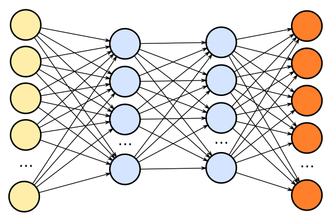
Next, I consider deep neural networks. Where artificial neural networks have a single hidden layer, deep neural networks have multiple hidden layers. Because of the complexity multiple hidden layers adds to the model, deep neural networks are better at some tasks than simple neural networks. However, their added complexity makes them more difficult to train.

Last, I discuss convolutional neural networks. Again, this is a variation of a simple neural network. A benefit to using a convolutional neural network is that it is designed to better handle image and speech recognition tasks. Instead of hidden layers, convolutional neural networks have a convolutional and pooling layer. It is because of these layers that convolutional neural networks are preferred for image and speech recognition.  
Thank you for following me on this series of machine learning blog posts. I haven’t even scratched the surface of everything I could talk about with machine learning, but I hope these blog posts have served as an introduction to a few of the topics in this field. It will be exciting to see where machine learning goes in the next 20 years and how it’ll change our lives for the better.

Two weeks ago, I introduced artificial neural networks. For this week’s blog post, I will be discussing convolutional neural networks. Like deep neural networks, as discussed in last week’s blog post, convolutional neural networks are related to artificial neural networks. For the sake of not repeating myself too much, I would strongly suggest looking back over my blog post on artificial neural networks and deep neural networks before reading the rest of my post.

The benefit of using a convolutional neural network over other types of neural networks is seen when attempting to build a model to do image recognition tasks. The structure of convolutional neural networks is similar to the basic neural network. It has input and output layers made up of nodes, each node with their own weight. However, if one tried to use a simple neural network for image recognition tasks, there would be too many weights for the model to work efficiently or accurately. As mentioned in this blog, if working with a 32×32 image, which is pretty small, and use only 3 color channels, there would be 3072 weights for a single node in the first layer of the neural network. For larger images, the number of weights only gets larger and harder to handle.

So, what exactly makes convolutional neural networks so good for image recognition tasks? These neural networks assume their inputs are always going to be some type of image, so ways to specially handle images can be built into the model. To define the model generally, convolutional neural networks take three dimensional input, the image, and produces a single vector, the classification for the image. The width and height of the input image are two of the dimensions, with the color values being the third dimension. In between the input and output layers there are two layers different than those in a simple neural network:  a convolutional layer and a pooling layer. The convolutional layer has a set of filters than can detect features in the image (an edge of a face, for example). The pooling layer divides the input image into smaller regions, and chooses the most important feature in that region to keep, discarding the rest. This approach is called max pooling, but there are other types of pooling.

For example, if one were trying to build a model to recognize animals, the model would be trained on a variety of animal pictures. To test its ability to recognize animals, give the model a new image of an animal it has seen before. The model’s output will be a vector with its prediction of what type of animal it will be, where each index in the vector represents a different animal.

Since this is the last blog post with a specific topic, next week I’ll be concluding this series of blog posts with a summary of each blog. Then, I’ll discuss some interesting new applications of machine learning and why it’s quickly becoming an important part of many non-computer science related fields.

Last week, I introduced artificial neural networks. For this week’s blog post, I will be discussing deep neural networks, which are closely related to artificial neural networks. If you haven’t read last week’s blog post, artificial neural networks have three main parts: an input layer, an output layer, and a hidden layer. Each layer is made up of nodes. The difference between artificial neural networks and deep neural networks is that deep neural networks have multiple hidden layers. However, it is important to note that the more hidden layers a deep neural network has, the harder it is to train the network.

Deep neural networks are useful because they allow for more learning within each hidden layer, despite difficulties with training deep neural networks with many hidden layers. Deep neural networks are a relatively recent development in machine learning. Why didn’t people try to make deep neural networks sooner? The main problem preventing people from making deep neural networks popular was efficiently training a deep neural network. However, with relatively recent advances, training a deep neural network has become easier.

The image above is an example of a deep neural network. The yellow/cream circles are the input layer and can contain an arbitrary number of nodes. The blue circles represent two hidden layers. Note that even though this picture displays two hidden layers, it’s possible to have many more hidden layers than just two. Again, the hidden layers can have an arbitrary number of nodes. The orange circles represent the output layer, or to put it simply, what the model is predicting. For example, for a DNN to predict weather, the input layer could contain temperature, humidity, rainfall, and wind. The hidden layers would do transformations on the input layer (or the previous hidden layer) until the output layer is reached. At that point, the model is ready to predict the weather as rainy, sunny, or cloudy. The arrows between each layer represent vectors. These vectors are the information passed and modified between each layer.

Deep neural networks can be trained using backpropagation. An input vector is fed through the model, layer by layer, until the output layer is reached. Then the output from the model is compared with the desired test output (see my blog post on data preparation about train, dev, and test sets for more info about training). Then, using a loss function to determine how right or wrong the model’s output was, the model changes its weights to minimize the loss function. We want to minimize the loss function because the smaller the loss, the more accurate predictions the model will produce. Weights are values associated with each node that change a node’s input vector. This process of calculating loss and changing weights is backpropagation.

Next week, I will discuss convolutional neural networks, another spin-off of artificial neural networks.

The image of a deep neural network used in this post can be found at https://blog.eduardovalle.com/tag/deep-learning/.

This week I will discuss the first machine learning model in this series of blog posts, neural networks.

When you google the definition of a neural network, google will respond with “a computer system modeled on the human brain and nervous system”. Neural networks may have been inspired by the human brain, but that is where the similarities end. The name “neural network” comes from the model having layers made up of nodes. The nodes were inspired by neurons in the brain, and links between neurons were inspired by synapses, hence “neural network”. Between you and me, the people to invent neural networks were probably looking for a catchy and scientific sounding name.

Neural networks first appeared in the early 1950’s when computers first started being created. In the 1990’s and early 2000’s, neural networks became popular as a machine learning tool and were beginning to be commercially viable. Even today, neural networks are still used. Applications of neural networks include classification, complex nonlinear function approximation, and data processing. Of course, neural networks are not the only model one can use in machine learning. There are support vector machines, decision trees, clustering, and so on. However, I will only discuss neural networks and some variations of neural networks in this series of blog posts.

The following image is an example of a simple neural network.

On the left, with red circles, is the input layer. Input layers take data as input, then pass it on to the hidden layer. Each circle is different data. For example, if the model was going to predict the weather for tomorrow, three inputs could be temperature, humidity, and wind. On the right, with green circles, is the output of the neural network. Sticking to the weather example, two outputs of the model could be rainy or sunny. In between the input and output layers is the hidden layer. The job of the hidden layer is to process, or transform, the input into a format the next layer can use. In this case, the next layer is simply the output layer. Neural networks can also have multiple hidden layers. These types of neural networks are called deep neural networks. The vectors between the layers represent transformations the data undergoes from layer to layer.

The amount of nodes in each layer varies from model to model. In the case of the input layer, its size may change as the amount of data used for input increases. The size of the output layer changes based on what the model was designed to predict. In this sense, neural networks are like people. They come in all shapes and sizes, and there is no perfect one for all situations.

Next week, I will discuss deep neural networks, a variation on neural networks, and how they compare to neural networks. As mentioned previously in this post, deep neural networks are simply neural networks with more hidden layers.

The image used in this post can be found at https://en.wikipedia.org/wiki/File:Colored_neural_network.svg.