In the the introduction to this blog, we discussed some of the incredible advances in the field of artificial intelligence in recent years. Using the tic-tac-toe vs. Go analogy for describing problem complexity, we disassembled the traditional “rule-based” approach to creating artificial intelligence and introduced the concept of “bottom-up” learning: a family of algorithms that learn to make decisions based on seeing massive amounts of data and learning by example. The bottom-up paradigm has become the backbone of deep learning, and is almost single-handedly responsible for the more recent A.I. renaissance.

In the first post, we stepped back in time to analyze one the first attempts at creating an algorithm that truly embodied the bottom-up paradigm: Frank Rosenblatt’s perceptron. Though Rosenblatt’s implementation was actually a piece of hardware, it gave birth to the connectionist paradigm and sparked questions about the relationship between the architecture of the perceptron and that of the human brain.

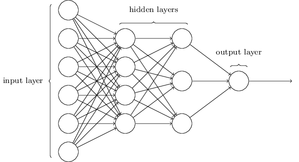
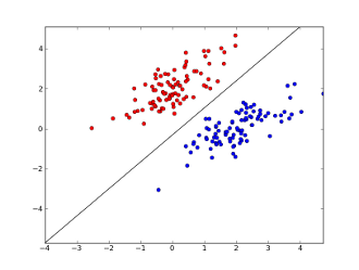
We addressed the issues with Rosenblatt’s perceptron (e.g. lack of hidden layer) in “Neural Networks and Gradient Descent”, and demonstrated how neural networks resolve these problems. We explored the universal approximation theorem, and showed that given enough nodes in a hidden layer, a single hidden layer neural network can theoretically approximate any function. This was a tremendous step forward from the perceptron’s inability to model the XOR function, and we discussed how researchers attempt to optimize neural networks via the gradient descent algorithm.

By the fourth post, “The Genesis of Deep Learning”, we had finally touched on the buzzword, “deep learning”. A natural extension of adding the single hidden layer to Rosenblatt’s perceptron, adding multiple hidden layers in turn added even greater computational power to the neural network. This introduced the need for the backpropagation algorithm, which allowed deep models to efficiently learn just like their shallower parents. With backpropagation we introduced the vanishing and exploding gradient problems, computational graphs, and went into greater detail on gradient descent and how vectors of partial derivatives are applied to weights in a neural network.

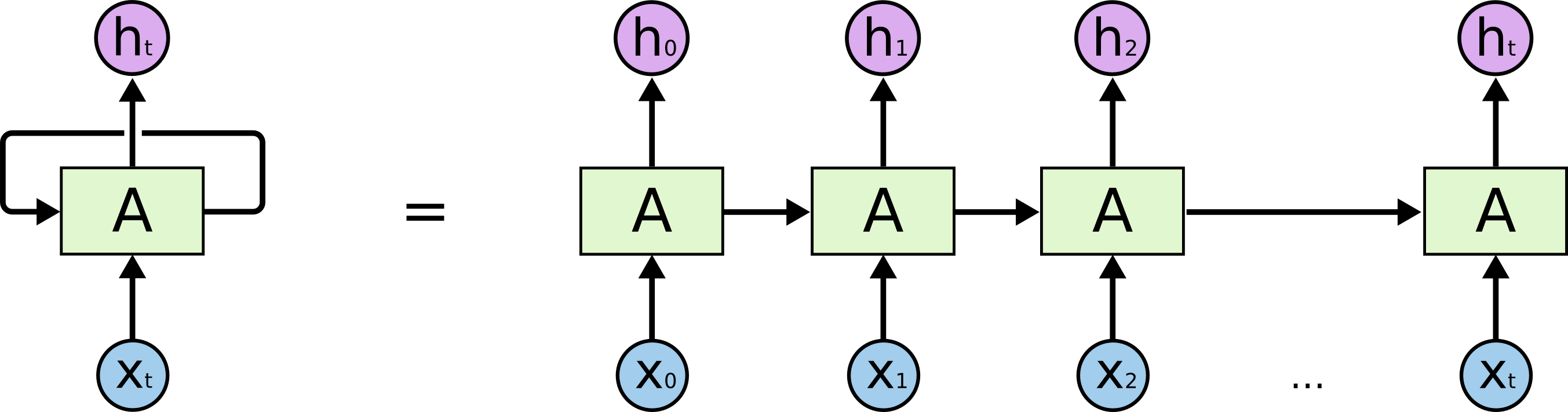
That was still just scratching the surface of what deep learning has really become. In “Learning Through Time”, we introduced a specialized form of deep neural network, the recurrent neural network (RNN). RNNs are fantastic models for processing sequential data, and we discussed how exactly RNNs are able to consume information over time. With the additional dimension of time thrown into the mix, we discussed backpropagation through time, and how training RNNs differs from training vanilla DNNs. We hinted at applications, but didn’t discuss how RNNs are used in modern A.I. applications.

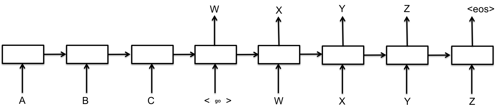
In the last post, we introduced the sequence-to-sequence model (seq2seq), an extension of the RNN, and showed how RNNs can be used to digest sequences, compressing them into single real-valued vectors of arbitrary size. We demonstrated how useful this train can be in natural language processing, where a summary vector can be used to generate incredibly natural-sounding language translations. The seq2seq machine translation algorithm revolutionized Google’s translation service overnight, and is still being improved upon to include a wider variety of languages.

Over the last few weeks, we’ve seen how neural networks evolved over time, starting as simple pattern classifiers and moving on to incredible tasks like language modeling and machine translation. This is far from a comprehensive tour of the world of machine learning, and just scratches the surface of what modern neural networks to do. These models are changing our world every day, and will soon be ubiquitous in our society. Everyone should have at least a basic understanding of the A.I. tools that we use everyday, and I hope that this blog has provided its readers with at least a working knowledge of deep learning.

Last week we discussed recurrent neural networks (RNNs), powerful models that are able to process sequential data such as speech, text, video, etc. We outlined the basic structure of an RNN, and how they can be trained via unrolling and backpropagation through time. At the end of last weeks post, we hinted at the fact that RNNs don’t always necessarily need to generate an output vector, and that in fact, the hidden states of recurrent neural networks can be utilized to assist even more sophisticated types of models. This week, we’ll discuss possibly the most well-known type of such models, the sequence-to-sequence neural network (seq2seq).

At the heart of these models are two vanilla recurrent neural networks, but what makes the seq2seq model special is the way that these two RNNs interact. Though seq2seq models can be used to process any kind of sequential (or even non-sequential, if you’re clever) data, as an example we will focus on processing natural language. So, just like last week, imagine that the input to our model is the simple English sentence, “I go.”. The input is broken up into three tokens: [“I”, “go”, “.”]. Each of these tokens is turned into a vector, and fed into a standard RNN (unrolled for 3 time steps) which applies the proper transformations and generates a final hidden state for the sentence. Now, with a standard RNN, we would generally use the final hidden state to generate some sort of output. Instead, what if we pass the final hidden state of this RNN to another RNN? Such a model is illustrated in the following figure:

Figure 1: Seq2Seq Architecture

Imagine that A,B, and C correspond to the three tokens we passed the original RNN (the encoder). The second RNN (the decoder) receives the final hidden state from the encoder, and takes in the special <GO> symbol as its first input. At each time step, the decoder outputs either a token or the special <EOS> (end of sentence) symbol which it uses to determine when to stop outputting tokens. Because the decoder receives previous hidden states and its own previous output as input at the next time step, it is deciding what kind of token to output based on what information it has previously extracted from the encoder’s final hidden state. All of this is very abstract, and we’ve really only outlined the skeleton of seq2seq models. So what are they good for? What happens to the sentence we input to the decoder?

Imagine that instead of the decoder outputting [“W”, “X”, “Y”, “Z”, “<EOS>”], it had actually output [“Je”, “vais”, “.”]. In French, that sequence of tokens means, “I go”. The seq2seq model has one very important application: it’s incredibly good at translating natural language languages. In September 2016, Google revealed that they would be using seq2seq models to revitalize the Google Translate service. Neural Machine Translation, as they called it, dramatically increased the fluency of the sentences output by Translate, and translations instantly become more natural and logical.

Figure 2: Example of Neural Machine Translation

So how is this possible? How can throwing two RNNs in a line lead to near-human level translations? We will address this question in next week’s post when we discuss embeddings and the power of high-dimensional space!

Sources:

https://www.tensorflow.org/tutorials/seq2seq

https://blog.google/products/translate/found-translation-more-accurate-fluent-sentences-google-translate/

Last week we talked about the birth of deep learning, the benefits of adding multiple hidden layers to a neural network, and how Paul Werbos applied the multivariable chain rule to his “backpropagation” algorithm to train deep neural networks. The advent of backpropagation allowed researchers to design far more complex architectures than they were previously using, and it was found that the algorithm was relatively resilient to complex models. This week, we’ll be talking about recurrent neural networks (RNN), a neural network architecture designed to process sequential input such as speech or video. RNNs are incredibly powerful, and have been directly responsible for a good number of breakthroughs in complex domains in recent years. Andrej Karpathy has a fantastic post about the numerous applications of RNNs, but here we’ll focus on the theory and history of RNNs.

Though the original inventor of the RNN is widely debated, most experts in the field agree that this architecture originally rose to popularity during the 1980’s. It was shown to be Turing complete, meaning that a properly trained RNN could essentially simulate anything that can be encoded as an algorithm. Realizing the significance of this, hundreds of papers came out during the late 80’s showing novel applications of RNNs to just about everything. A high level overview of the model is presented below:

While the image on the left is an accurate representation of an RNN, it is often more helpful to think of the RNN in an “unrolled” state, pictured on the right. Here, each X_t corresponds to an input vector that is part of the overall sequence of inputs. For example, if this RNN were a language model, each input vector might correspond to a word in a sentence. The input vector is multiplied by an input weight, which is shared between all time steps (as demonstrated in the figure on the left) to create the hidden state of the RNN, the box labeled A. This hidden state is also a vector of arbitrary dimension, which can be thought of as maintaining an abstract representation of the sequence. Note that A is not just a transformation of the input vector, but also of the previous hidden state. By multiplying the previous state vector by a recurrent weight and combining it with the input vector, the RNN can essentially maintain a working short-term memory of what information it’s seen in previous inputs.

In this diagram, the RNN is generating an output, H_t, at every time step. Just like with the input weight, the output weight is shared by all steps in the sequence, and is multiplied against the hidden state vector to generate some output vector. This could be a single number, used to guess a speaker’s age based on a sentence they’ve spoken, or a probability distribution, used to recognize a paragraph as being written by a certain author. However, it is not necessary that the RNN generate an output at every time step. It is entirely possible that the RNN doesn’t output anything until the entire sequence has been processed, or more interestingly, the output might be the hidden state itself, unmodified by an output weight. We’ll discuss an application of this idea, the sequence-to-sequence model, in next week’s post!

Last week we talked about simple single hidden layer neural networks and gradient descent. The addition of hidden layers allowed the model to implicitly map the input feature vector into a higher dimension without all of the computational complexity of actually exploring the high dimensional space. Gradient descent is an algorithm that improves the performance of a model by computing vectors of partial derivatives, which it uses to “descend the error bowl” and reach an optimal point in the space of the neural networks weights. Generally, the error that gradient descent attempts to minimize depends on the task at end: regression or classification. Regression tasks involve outputting vectors of real numbers; essentially predicting points in arbitrary dimensions. This is just like the type of linear regression seen in many introductory statistics classes.

Given a dataset (represented by the blue points), a neural network optimizing on a regression task would try to approximate a function (represented by the red line) that best fits the dataset. Alternatively, a neural network may also be used as a classifier, outputting a probability density function that is compared to a datapoint’s label.

Typically, the loss function for regression is mean squared error, and cross-entropy for classification. However, as long as the loss function is differentiable, neural networks can really be trained to approximate anything that can intuitively be thought of as a function.

After researchers saw how the addition of a hidden layer massively increased the expressiveness of perceptrons, they began experimenting with varying numbers and sizes of the hidden layers in neural networks. The results were astounding, and this is when “deep” neural networks really came into the limelight. The idea was that extra hidden layers allowed the model to learn more abstract representations of the data, which would be far more beneficial than the feature vectors that a human could provide the model as input. In theory, each layer would learn to extract a different set of features, specializing to focus on the parts of the input that would be most beneficial to subsequent layers. These deep architectures allowed neural networks to perform such tasks as handwriting recognition and language modeling with far greater accuracy than in the past.

However, training these models was far more problematic than expected. Gradient descent was still an adequate algorithm for computing the vectors of partial derivatives, but the extra hidden layers introduced an interesting problem: the deeper a network was, the harder it was to train. This was because training earlier layers was essentially impossible with traditional applications of gradient descent. This problem was solved by Paul Werbos, who introduced the backpropagation algorithm for training neural networks. Essentially a well-marketed application of the multivariable chain rule, backpropagation calculated the error of the network, just as in vanilla gradient descent, but then distributed the “blame” for the error amongst all of the weights that contributed to the final result.

Above is an example of the “computational graph” that demonstrates how the partial derivatives in a neural network are applied in backpropagtion. This algorithm became crucial to the success of more complicated architectures, and allowed deep learning to take off. Next week, we’ll discuss recurrent neural networks and backpropagation through time.

Last week we talked about a primitive cornerstone in the connectionist paradigm, Frank Rosenblatt’s Perceptron. Despite it’s similarity to modern, more successful connectionist models, its lack of expressive ability ultimately led to its downfall. After Marvin Minsky, a prominent leader in the AI community at the time, personally decried the machine for being unable to model the simple exclusive-or (XOR) function, connectionist models rapidly fell out of fashion. The field returned to the top-down approach, using rule-based languages such as Prolog and LISP to create so-called “expert systems”: programs that could reason through relatively complex problems by incorporating domain-specific knowledge with the relational reasoning that is ubiquitous in rule-based programming. Essentially, the field of artificial intelligence had returned to if-else statements and glorified flowcharts.

Figure 1: Architecture of an “expert system”

There were two major breakthroughs that brought connectionist AI back from the grave: the McCulloch–Pitts (MCP) neuron and the addition of a hidden layer. Together, these mechanics form the skeleton for what we now refer to as a neural network. The hidden layer is simply an intermediate stage between the input and output of a neural network that allows the model to implicitly map the input data into high-dimensional space and create a more abstract representation of the features. Working in a higher dimension means that the feature-space of the hidden layer is far richer, meaning that the network will have a far greater expressive power. The MCP neuron is an architecture vaguely based on the structure of neurons in the brain. In the brain, networks of neurons interact in a binary way: they either fire or they don’t fire. In the MCP artificial neuron, “firing” is done with an activation function. These functions are generally sigmoidal, and squish the output of a hidden layer.

Figure 2: Example of a sigmoidal function (logistic sigmoid)

Mathematically, these activation functions introduce non-linearity into the system, allowing neural networks to generate complex, non-linear decision boundaries (as we saw in last week’s post). The activation shown above isn’t completely binary, but it does force values to fall between 1 and 0. There are other types of activation functions, and depending on the architecture of the neural network, a vanilla logistic sigmoid may not be the best choice. We’ll cover types of activation functions when we talk about Deep Learning. So with the addition of hidden layers, we end up with an architecture similar to this:

Figure 3: A simple neural network

The edges represent multiplication by a weight matrix and the addition of a bias vector. After each hidden layer, an activation function is applied to the elements of the hidden vector. In the above example, the output is a scalar.

So how does such a complicated model actually learn? The secret is in the type of operations that compose the network– every single one is differentiable. For a model that is just composed of an input and output layer, optimizing the weights is a simple process: we calculate the derivative of the entire model given its output error to produce a gradient. The gradient is a vector that represents the direction of steepest ascent for a function. So if we add the negative of the gradient to our model’s weights, the entire network will approach a more optimal configuration. Imagine a giant, high-dimensional bowl that represents how bad our model is, and a ball at the top of the curve is our model’s initial configuration. We want to make our model, so we want to minimize it’s error. This is analogous to the ball rolling down the sides of the bowl until it reaches it’s optimal location at the lowest point in the center. This algorithm is called gradient descent, and is the source of a neural network’s ability to learn. Next week, we’ll discuss the genesis of deep learning, and how gradient descent works with deeper models.

Source:

http://www.igcseict.info/theory/7_2/expert/files/stacks_image_5738.png

https://upload.wikimedia.org/wikipedia/commons/thumb/8/88/Logistic-curve.svg/320px-Logistic-curve.svg.png

In 1957, psychologist Frank Rosenblatt submitted a report to the Cornell Aeronautical Laboratory in which he claimed that he would be able to, “construct an electronic or electromechanical system which will learn to recognize similarities or identities between patterns of optical, electrical, or tonal information, in a manner which may be closely analogous to the perceptual processes of a biological brain.” Specifically, Rosenblatt was interested in building a “photoperceptron”: a probabilistic system that would receive images as input and be able to determine which class they belong to. He imagined the perceptron would differentiate between different shapes, regardless of their scale, color, orientation, etc., and that it would learn to do this by observing thousands of images and their associated labels. This idea was the genesis of “bottom-up” learning, and we now recognize Rosenblatt’s perceptron as the grandfather of one of the most effective machine learning algorithms that we use today: the deep neural network (DNN).

However, Rosenblatt’s model was not nearly as successful as he had hoped. He envisioned the perceptron not as an algorithm implemented in software, but as a custom piece of hardware. Because of this, the machine would only accept a 400-pixel image as input and could not generalize to other problems. Furthermore, the mathematical model itself received criticism for being inflexible and crude. As the perceptron did nothing more than multiply a feature-vector by a set of adjustable weights, it could only learn to model linear functions– essentially, Rosenblatt had implemented high-dimensional logistic regression. Now, logistic regression is a perfectly suitable algorithm for many classification tasks, assuming the true underlying distribution of classes is linearly separable. For example, if pictures of squares and circles could be mapped into a space in which they are distributed as in the picture below, a perceptron could (theoretically) learn a linear decision boundary to perfectly classify these data points.

If the underlying function that determines the class distribution is more complex, a linear decision boundary can never accurately model the proper decision boundary. Imagine a perceptron trying to model a sinusoidal function: instead of generating a smooth curve, the model would likely realize that the best it could do would be a perfectly horizontal line running through the center of the curve. Obviously, this is less than ideal. When the underlying function is non-linear, we want a decision boundary that can model this relationship (as pictured below).

This limitation essentially buried the perceptron, and the connectionist paradigm of A.I. development screeched to a halt. Some years later, it would be discovered that adding a hidden layer to the perceptron would allow it to learn arbitrary functions. The idea was that instead of simply multiplying an input vector by a set of weights to get a classification, the first set of weights would implicitly map the input vector into a higher dimension (similar to kernel methods), and that a second set of weights would map this higher-dimensional representation of the data to its corresponding class. Given that the hidden layer was large enough, this gave the multilayer perceptron (MLP) the expressive power it needed to approximate tricky non-linear decision boundaries and take on far more complicated tasks. This marked an incredible leap forward for connectionist models, and MLPs enjoyed a decent amount of popularity in the following years. However, the MLP was still far from achieving its true potential, and researchers wouldn’t realize this until they began to explore even deeper models in the early 80’s. Next week we’ll explore the benefits of additional hidden layers and the birth of deep learning.

Sources:

http://blogs.umass.edu/brain-wars/files/2016/03/rosenblatt-1957.pdf

http://datascience.stackexchange.com/questions/1253/why-are-nlp-and-machine-learning-communities-interested-in-deep-learning

“Isn’t it funny how day by day nothing changes, but when you look back, everything is different?” – C.S. Lewis

For decades, the ancient Chinese game of Go has been the so-called “unsolvable” benchmark to push artificially intelligent (AI) machines to their limits. With the standard 19×19 tournament board containing 361 intersections and allowing for more possible board configurations than there are atoms in the known universe, it’s understandable that a computer might have a bit of difficulty planning its next move. The magnitude and flexibility of this game make all traditional AI methods essentially useless, and enumerating and evaluating each possible move is prohibitively inefficient for even the most powerful supercomputers. But in March of 2016, Google solved it. Well, maybe that’s a bit of an overstatement. Regardless, their “AlphaGo” algorithm had defeated world-champion 9-Dan Go player Lee Sedol 4-1, a task that was completely unheard of just a few years earlier, and even by the most optimistic estimations wasn’t expected to happen for at least 10 more years. In that same year, we saw similarly intelligent algorithms make a variety of break-throughs: WaveNet generated almost indistinguishably human-like synthetic speech from text, one model learned to play Atari games solely from visual input, another became a super-human lip reader, and the Google Translate service improved by an order of magnitude seemingly over night.

All of these incredible feats marked tremendous leaps forward in the field of artificial intelligence, but each and every one of them have one thing in common: they aren’t really intelligent at all. At least by what you might call a “standard” definition. AlphaGo doesn’t know that it’s playing a game, what a game is, or even what a Go board looks like. Similarly, the lip-reading algorithm doesn’t know anything about words, what lips are, or how to speak itself. Yet somehow, these models are performing at superhuman levels with absolutely zero domain-relevant knowledge. This is thanks to a relatively recent (and incredibly successful) paradigm shift in the field of artificial intelligence. For years, researchers and programmers have attempted to create intelligent machines by teaching them immensely complex sets of rules. For a good number of applications, this is a perfectly fine approach. If you want an AI to play tic-tac-toe without losing, you simply program it to block its opponent whenever they have two pieces in a line. If you want a robot to scoot around without running into anything, simply have it turn whenever it detects something in its path. But what if we want to, say, recognize a handwritten digit in an image?

Suddenly, everything becomes much more complicated. Our model’s rules would need to account for an incredible amount of variance to be able to handle the types of noisy, real-world data that humans deal with on a daily basis. That makes for one long “else if” chain. Instead, we can craft our models from the bottom up, letting them learn these rules for themselves by viewing a massive number of examples. As it turns out, this simple idea is responsible for almost all of the unbelievable achievements in AI that we’ve seen in the last decade. Self-driving cars, face-recognition, and recommender systems all rely on an incredibly powerful realization of the “bottom-up” approach: the artificial neural network (ANN). By using techniques from calculus, linear algebra, and statistics, ANNs can be “trained” to approximate incredibly high-dimensional functions that simulate abstract understanding and can be applied to complex problems like computer vision and natural language processing. They’ve revolutionized the field of machine learning and led us into an AI renaissance that will likely continue for decades.

So how did we get here? Just a decade ago this would have sounded like the stuff of science fiction, and now even top researchers have a hard time keeping up with the rate of progress (but they’re working on it). In this blog, we’ll dive into the history of artificial intelligence and explore what exactly led us to this incredible explosion of progress. We’ll analyze multiple types of neural networks and their uses, introduce the work of big names in the industry, and discuss applications of this amazing algorithm. Next week, we start off with an introduction to the deep neural network (DNN)!